Sampling Part 1: Basics of Sampling
- Nov 2, 2021
- 5 min read
How Can We Learn Anything about the Whole Country by Asking Only 1000 People?
Almost all adults have experienced voting. Based on that experience and common sense, we could conclude that measuring any phenomenon at the country level requires asking all country's adult citizens about the phenomenon. That is correct, but only if we must have the exact figure. However, if we can tolerate some predetermined amount of error, we can opt for a much more feasible research design – using a sample to make inferences about the population. Unfortunately, the logic behind making inferences about the population (link za ab testing) based on the sample is not intuitive. Furthermore, researchers frequently have a hard time convincing their audience of the relevance of their results for the population. This post aims to provide basic knowledge about sampling and enhance confidence when reading or communicating survey results.
What exactly is the population?
The population represents all entities (e.g., people) that we are interested in when exploring a particular topic. That could be all adults, but also a much narrower group, depending on the goal of our study. For example, we could be interested only in people planning to buy a car next year, or only in women with dyed hair who use conditioner at least twice a week. A measure that we want to estimate in the population is called a parameter. Interviewing all of the members of the population that we are interested in is very expensive and time-consuming. That is why we use surveys on the part of the population – a sample. Common logic says: „the more significant portion of the population we include in our sample, the more reliable the result we are going to get. “However, things are a little more complicated than that. A method of extracting a sample from a population is equally important as its size.
Random samples
In the context of sampling, randomness means that every population member has an equal chance of being selected into the sample. Why is that important? If the population members with specific characteristics are more or less likely to be included in the sample, that introduces systemic bias.
For example, if doing an internet survey, the younger people are usually more likely to answer the questions. This inequality can skew our sample towards having a more significant proportion of young people than our population. Young people may hold different opinions and have different preferences regarding the study topic than other population segments, and here we are - making incorrect conclusions because of a biased sample. We sampled randomly, but our sampling frame or the register of the people from which we selected our sample did not represent the population in which we were interested.
The central limit theorem and the basics of statistical inference
We start with the assumption that no sample is perfect. The result that we get today, on one particular sample, is slightly different from what we could get tomorrow if we drew another sample from the same population. So, our estimate of the parameter (population value) will be slightly off every time we make a conclusion based on a sample. Because of this, it’s essential to be able to estimate how much we are wrong. How much we can go wrong depends on the variability of the phenomena we are measuring (for more detail, look at our post about statistical significance). For example, if we want to determine the average number of hand fingers in the population, we cannot go too wrong with almost any sample (unless we get too many yakuza members in it). On the other hand, if we want to measure average height in the population, we have to be much more circumspect, given that people differ significantly in height.
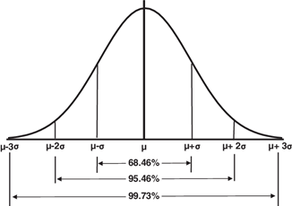
Every time we draw a sample, the mean of the characteristic of interest that we calculate from it will be a little different. So, we accept that we might never nail the actual population mean, but we do expect to be somewhere close to it. If we drew many random samples from the same population, the sample mean would sometimes be below the population mean and sometimes above it. Here comes the exciting part. If we take enough (>100) random samples that are large enough (>30 population members in each sample), those sample means will get the bell-shape of a normal distribution, with the population mean in the center. Somewhat surprisingly, this rule works even in the case of the not normally distributed measures. This phenomenon is known as the central limit theorem, and it is one of the pillars of statistics.
What is the standard error?
You can say, „Nice trick, but how can we use it?“. Well, a normal distribution has some handy features. For example, we know that, in normally distributed data, ~95% of cases lie between -2 and +2 standard deviations.
In theory, if we took >100 samples and calculated the mean of every sample, we would get a (normal) distribution of the sample means. Then, we could calculate the standard deviation of this distribution, usually known as the standard error of the mean. That would enable us to conclude how distant every sample’s mean is from the population mean. But, of course, we will never do 100+ surveys on the same topic. But, clever statisticians came up with a way to estimate standard error using the standard deviation we calculate on our (one and only) sample. We can calculate the standard error as follows:
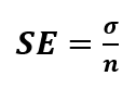
Where σ is the standard deviation found in our sample, and n is the sample size.
Confidence intervals
Based on the standard error, we can calculate the boundaries, known as confidence intervals, where we expect that the population result lies. This is how we get our confidence intervals:
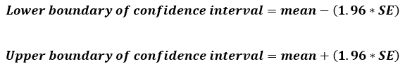
When we say that we expect the population result to lie somewhere between the lower and upper boundary of the confidence interval, it highlights the fact that we are not sure about the exact value of the population result. We expect that the population mean lies between the boundaries with 95% confidence[1]. We will never report the estimate of the exact value in isolation. For example, we will never say that we estimate that the population high mean is 172.36 cm, but instead say 172.36 with a 95% CI [169.48, 175.24].
Let’s think about the above equations for confidence intervals again. The lower the standard error is, the narrower the confidence intervals are. The narrower the confidence intervals are, the more precise our prediction is. Confidence intervals that are too broad will not be useful to someone who wants to use our results. For example, a clothes manufacturer will not be pleased if we tell them that the height of an average man is somewhere between 151. 23cm and 188.52cm. Too broad confidence intervals indicate is that the measure varies widely in the population. And while we can not change that, we can counter it by drawing a larger sample. Continue reading our second post on sampling to learn more about determining the correct sample size for your study.
[1] If we wanted to calculate 99% confidence interval we would replace 1.96 with 2.58 in the equation above.


Comments